Image analysis

Table of Contents

Introduction
Data management
Data augmentation

Introduction

In previous lessons, we’ve worked extensively with tabular data—structured datasets where each row represents an observation and each column represents a feature. These datasets are typically easy to represent and analyze using tools like pandas, scikit-learn, and various statistical models.

However, images are fundamentally different in both structure and content. Instead of rows and columns of explicitly labeled features, an image is a grid of pixel values—typically in 2D for grayscale or 3D for color (height × width × channels). For example, a color image of size 224×224 pixels with 3 color channels (RGB) contains over 150,000 raw values, none of which are labeled with human-interpretable features like «age» or «income».

This difference leads to several important challenges:

High Dimensionality: Images contain many more features (pixels) than typical tabular datasets, which increases computational complexity and the risk of overfitting.
Spatial Structure: Nearby pixels in an image are often related, forming edges, textures, and patterns. Tabular models generally do not capture such local dependencies.
Semantic Gap: The relationship between raw pixels and meaningful concepts (like a cat, a face, or a traffic sign) is complex and non-linear, requiring sophisticated models to bridge this gap.

Because of these challenges, we need image-specific models, most notably Convolutional Neural Networks (CNNs), which are designed to exploit the spatial and hierarchical structure of images. These models learn to recognize patterns such as edges, shapes, and eventually objects, by processing images in layers of increasing abstraction.

In this module, we will explore how to work with image data. To do so we will use again PyTorch.

Memory Constraints with Image Datasets

Unlike tabular data, where datasets can often be loaded entirely into memory (e.g., a CSV with thousands of rows and columns), image datasets present significant memory challenges. Images are high-dimensional data: a single 224x224 RGB image contains 224 * 224 * 3 ≈ 150,000 values (pixels), each typically stored as a float32 (4 bytes), resulting in about 600 KB per image. For a dataset of 1 million images, this would require approximately 600 GB of RAM, which exceeds the capacity of most systems.

This memory limitation fundamentally changes how we work with image data:

Batch processing: We use data loaders that load images in small batches (e.g., 32-128 images at a time) rather than the entire dataset.
On-the-fly transformations: Images are often resized, normalized, or augmented as they are loaded, avoiding the need to store preprocessed versions.
Iterative training: Models are trained using iterators that fetch batches sequentially, enabling training on datasets larger than available memory.
Efficient storage: Techniques like lazy loading from disk or using compressed formats help manage large datasets without overwhelming memory.

Data management

When training deep learning models with images, we don’t feed the whole dataset at once—unlike traditional machine learning with tabular data. Instead, we process images in batches: small groups of samples processed together.

A batch is a collection of samples (e.g., images and their labels) processed together in a single forward and backward pass. For example, instead of training on 1,000,000 images at once, we might process 32 images, update weights, then move to the next 32.

Why Batching?

Memory Efficiency: Batches make full dataset training feasible by processing only a subset at a time, fitting within GPU/CPU memory constraints (recall: 1M images = 600+ GB).
GPU Parallelism: Modern GPUs excel at parallel processing; batches leverage this by applying the same operation to many images simultaneously.
Gradient Stability: Computing gradients on a batch provides more stable estimates than single-sample updates, reducing training noise and improving convergence.

Key Relationship

For a dataset with \(N\) samples and batch size \(B\):

Iterations per epoch = \(\lceil \frac{N}{B} \rceil\) (number of batches)
Total iterations = Iterations per epoch × Number of epochs

Example: 10,000 images with batch size 32 = 313 iterations per epoch (each epoch processes all 10,000 images in 313 batches).

Terminology

Batch Size: The number of samples in a single batch (e.g., 32, 64, or 128). This is a critical hyperparameter—larger batches use more memory but train faster; smaller batches are more memory-efficient but noisier.
Epoch: One complete pass through the entire dataset.
Iteration: One update step; corresponds to processing one batch.

Example

In the following code, we will create a PyTorch MLP model similar to the ones discussed in the previous section. We will attempt to train it using the entire image dataset without batching, as you did in the previous leasons. To do so we will use a test image dataset: CIFAR-10.

CIFAR-10

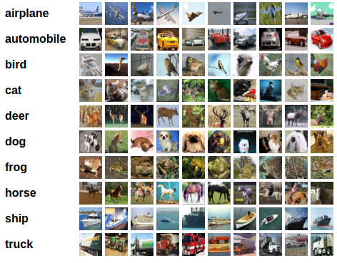
CIFAR-10 is a widely-used dataset for image classification tasks, containing 60,000 32x32 color images across 10 different classes (such as airplanes, cars, birds, etc.). Thanks to PyTorch and its torchvision library, we can easily access this dataset along with many other standard test datasets commonly used in machine learning research, you can explore the complete list of available datasets in torchvision.

To load an existing datset we need to use datasets and DataLoaders. These are two important objects for PyTorch and we will explain them in more detaill in a few minutes. For now we only need to untendertand that are how we load images to use it for

[ ]:

import torch
import torchvision
import torchvision.transforms as transforms

# Load CIFAR-10 dataset
transform = transforms.ToTensor()
trainset = torchvision.datasets.CIFAR10(root='./data', train=True, download=True, transform=transform) # download must be True if is the first time you execute this notebook

# Load the entire dataset into memory
trainloader = torch.utils.data.DataLoader(trainset, batch_size=len(trainset), shuffle=False)
images, labels = next(iter(trainloader))

# Flatten images for MLP input
images = images.view(images.size(0), -1)  # Shape: (50000, 3072)
print(images.shape)

The output shape (50000, 3072) represents:

50000: The number of images in the CIFAR-10 training dataset
3072: The total number of pixels (features) per image. Since CIFAR-10 contains 32×32 RGB images, each image has 32 × 32 × 3 = 3,072 pixel values (three channels for Red, Green, and Blue). By flattening the images, we convert each 3D image (32, 32, 3) into a 1D vector of 3,072 features suitable for MLP training.

So now we will define a model as the one we used for tabular data.

Remember:

If we have 3072 input features the model must have this amount of input features.
Also take into account that if the task is more complex we need a bigger net. Therefore if we have a problem of around 4000 features we need a larger model!
Lastly, remember that the ouput must correspond to the number of classes in a classification task.

[ ]:

import torch
import torch.nn as nn

# Model definition. Here we have to define the layers and the activation functions between them.
model = nn.Sequential(
    nn.Linear(3072, 8000),
    nn.ReLU(),
    nn.Linear(8000, 8000),
    nn.ReLU(),
    nn.Linear(8000, 3000),
    nn.ReLU(),
    nn.Linear(3000, 1000),
    nn.ReLU(),
    nn.Linear(1000, 500),
    nn.ReLU(),
    nn.Linear(500, 100),
    nn.ReLU(),
    nn.Linear(100, 10)
)

WARNING: only execute this in a colab session!

[ ]:

model(images)

It’s important to note that CIFAR-10 is actually a relatively simple and small dataset compared to real-world image datasets. However, even with this modest dataset, loading the entire 50,000 images (approximately 600 MB of data) into memory and make the prediction can be problematic for training. This demonstrates why batching is essential in machine learning: it allows us to process data in manageable chunks, reducing memory requirements and enabling training on much larger datasets. In practice, modern datasets like ImageNet contain millions of images that would be impossible to load all at once into memory.

PyTorch is heavely built around the idea of batching. Let’s see what we have to change in the previous code to use it:

[ ]:

BATCH_SIZE = 10

# Load CIFAR-10 dataset
transform = transforms.ToTensor()
trainset = torchvision.datasets.CIFAR10(root='./data', train=True, download=True, transform=transform) # download must be True if is the first time you execute this notebook

# Load the entire dataset into memory
trainloader = torch.utils.data.DataLoader(trainset, batch_size=BATCH_SIZE, shuffle=False)
images, labels = next(iter(trainloader))

# Flatten images for MLP input
images = images.view(images.size(0), -1)  # Shape: (50000, 3072)
print(images.shape)

[ ]:

model(images)

We can see that now the prediction has been without delay of any kind. We can use this approach to train and to evaluate a complex machine learning model. Let’s dive into the what it is a dataset and a dataloader in PyTorch.

PyTorch Dataset and DataLoader

A Dataset in PyTorch is an abstract class that represents a collection of data samples. It defines how to access individual data samples and their corresponding labels. PyTorch provides built-in datasets like CIFAR-10, ImageNet, MNIST, etc., through torchvision.datasets.

A DataLoader is a wrapper around a Dataset that handles:

Batching: Groups multiple samples into batches for efficient processing
Shuffling: Randomly reorders samples during training (improves generalization)
Parallel loading: Loads data using multiple worker processes for faster I/O
Automatic padding/collation: Handles variable-sized samples

A DataLoader must return the input data and the ground truth we want to predict.

Efficiency: Batching enables vectorized operations on GPUs
Scalability: Can handle datasets larger than available RAM
Convenience: Handles indexing, batching, and shuffling automatically
Best practices: Follows PyTorch conventions for reproducible research

Previously we used already these two classes in the following code:

trainset = torchvision.datasets.CIFAR10(root='./data', train=True, download=True, transform=transform)
trainloader = torch.utils.data.DataLoader(trainset, batch_size=BATCH_SIZE, shuffle=False)

Each dataset has its unique parameters. Each dataloader has three main parameters:

batch_size: Number of samples per batch
shuffle: Whether to shuffle data (typically True for training, False for validation/testing)
num_workers: Number of parallel processes for data loading

Let’s play a little bit with this objects. We can use next(iter()) to obtain the following element of the trainset so we see how they are.

[ ]:

res = next(iter(trainset))
res

How many elements there are?

[ ]:

len(res)

What are they?

[ ]:

print(res[0].shape)
print(res[1])

An image and a class! Lets see the image:

[ ]:

from torchvision.transforms.functional import to_pil_image

to_pil_image(res[0])

In PyTorch, images are typically represented as tensors with a specific shape convention:

Single Image Shape: (C, H, W)

C: Number of channels (3 for RGB, 1 for grayscale)
H: Height in pixels
W: Width in pixels

Example: A standard RGB image has shape (3, 32, 32) - 3 color channels, 32 pixels tall, 32 pixels wide.

Let’s do the same but for dataloader

[ ]:

res = next(iter(trainloader))
res

[ ]:

print(len(res))
print(res[0].shape)
print(res[1])

[ ]:

batch, labels = res
to_pil_image(batch[0])

ImageFolder Dataset

The ImageFolder class from torchvision.datasets provides a convenient way to load images organized in a directory structure. It automatically infers class labels from the folder hierarchy:

root/
  class1/
    img1.jpg
    img2.jpg
  class2/
    img3.jpg
    img4.jpg

Each subfolder represents a class, and images within are assigned that class label. This is ideal for standard image classification datasets where your data is organized in a folder-per-class structure.

Data augmentation

PyTorch’s Transform API (via torchvision.transforms) provides a composable way to apply transformations to images during the data loading pipeline. The key component is transforms.Compose(), which chains multiple transformations together:

[ ]:

transform = transforms.Compose([
    transforms.Resize((128, 128)),
    transforms.RandomRotation(180)
])

Each transformation is applied sequentially to the data as it’s loaded, making it efficient and flexible.

[ ]:

batch_transformed = transform(batch)
to_pil_image(batch_transformed[0])

Many transformation exist in `PyTorch <https://docs.pytorch.org/vision/0.8/transforms.html>`__. This transformations usually are used for two reasons: preprocess the image (change the size for example) and data augmentation.

Data Augmentation is the technique of artificially increasing the size and diversity of your training dataset by applying random transformations (rotations, flips, crops, color jittering, etc.) to images. This is one of the most effective regularization techniques in deep learning because:

Improves Generalization: By training on diverse versions of the same image, the model learns more robust features and is less likely to overfit.
Simulates Real-World Variations: In practice, images come from different angles, lighting conditions, and perspectives. Augmentation helps the model handle these variations.
Effective Data Multiplication: You can effectively create hundreds or thousands of variations from a small dataset without needing to collect new data.

Example augmentations:

RandomRotation(30): Random rotations up to 30 degrees
RandomHorizontalFlip(p=0.5): 50% chance of horizontal flip
ColorJitter(brightness=0.2): Random brightness changes
RandomCrop(size=32): Random crops to the specified size

The dataset combines data loading, batching, and transformations in a way that makes data augmentation extremely efficient:

[ ]:

trainset = torchvision.datasets.CIFAR10(
    root='./data',
    train=True,
    download=True,
    transform=transform  # ← Transforms applied here!
)

trainloader = torch.utils.data.DataLoader(
    trainset,
    batch_size=BATCH_SIZE,
    shuffle=True
)

Why is this a superpower?

On-the-fly Augmentation: Transformations are applied during data loading, not during preprocessing. This means:
- Each epoch, the same images are transformed differently
- You get infinite variations of your data without storing them all
- Memory efficient: only need to store the original dataset once

Separate Pipelines for Train/Test: You can use different transforms for training (with augmentation) and testing (without augmentation):

train_transform = transforms.Compose([
    transforms.RandomRotation(30),
    transforms.RandomHorizontalFlip(),
    transforms.ToTensor(),
    transforms.Normalize(mean, std)
])

test_transform = transforms.Compose([
    transforms.ToTensor(),
    transforms.Normalize(mean, std)
])

Parallelization: DataLoaders can use multiple workers to apply transformations in parallel while fetching the next batch, making training faster.

This is why well-tuned data augmentation combined with DataLoaders is one of the most effective techniques for improving deep learning model performance without collecting more data.

Now it’s your turn to practice the Transform API and see data augmentation in action!

Objective: Create multiple transform pipelines and visualize how different augmentations affect the same image.

Tasks:

Create three different transform pipelines:
- weak_augmentation: Only basic transforms (Resize, ToTensor, Normalize)
- medium_augmentation: Add some augmentation (RandomRotation, RandomHorizontalFlip)
- strong_augmentation: Add aggressive augmentation (RandomRotation, RandomHorizontalFlip, ColorJitter, RandomAffine)
Load a sample image from the CIFAR10 dataset using each pipeline
Visualize the results

[ ]:

#TODO