Decision Trees, Random Forest and XGBoost

Table of Contents

1. Introduction

2. Decision Tree

3. Random Forest

4. XGBoost

5. Exercise

In this notebook we will use XGBoost. We need another library:

!uv pip install xgboost

"uv" no se reconoce como un comando interno o externo,
programa o archivo por lotes ejecutable.

from sklearn.datasets import load_wine
from sklearn.model_selection import train_test_split
from sklearn.tree import DecisionTreeClassifier, plot_tree
from sklearn.metrics import accuracy_score, classification_report
import matplotlib.pyplot as plt
from sklearn.ensemble import RandomForestClassifier
from xgboost import XGBClassifier

The dataset used is the Wine dataset, a classic dataset in machine learning containing chemical properties of wines and their corresponding classes.

Let’s load and prepare the data:

wine = load_wine()
X = wine.data
y = wine.target

We divide the data into train and test:

X_train, X_test, y_train, y_test = train_test_split(
    X, y, test_size=0.3, random_state=42
)

4. Decision Tree

A Decision Tree is a supervised machine learning algorithm. It works by splitting the data into smaller subsets based on feature values, forming a tree-like structure of decisions. Each node represents a decision based on a feature, each branch represents the outcome of that decision and each leaf represents a final prediction.

We can put the following parameters:

• random_state: ensures same tree each run.

• max_depth: limits how deep the tree can grow preventing the model from becoming too complex. If we use a small depth, the model is simpler and may underfit. If we use a larger depth, the model can become too complex and overfit.

• min_samples_split: minimum samples to split a node. If we use a higher value, there will be fewer splits and the tree is simpler. Otherwise, the tree becomes more complex. This value helps to control overfitting.

• criterion: It is a function used to measure the quality of a split. It usually takes «gini» or «entropy». Gini is more commonly used.

dt = DecisionTreeClassifier(random_state=42)

Let’s train with the training data:

dt.fit(X_train, y_train)

DecisionTreeClassifier(random_state=42)

In a Jupyter environment, please rerun this cell to show the HTML representation or trust the notebook.
On GitHub, the HTML representation is unable to render, please try loading this page with nbviewer.org.

Perform predictions on the evaluation set:

y_pred_dt = dt.predict(X_test)

Then, we evaluate the performance:

print("Decision Tree Accuracy:", accuracy_score(y_test, y_pred_dt))
print(classification_report(y_test, y_pred_dt))

Decision Tree Accuracy: 0.9629629629629629
              precision    recall  f1-score   support

           0       0.95      0.95      0.95        19
           1       0.95      1.00      0.98        21
           2       1.00      0.93      0.96        14

    accuracy                           0.96        54
   macro avg       0.97      0.96      0.96        54
weighted avg       0.96      0.96      0.96        54

We can visualize the decision tree:

plt.figure(figsize=(15,10))
plot_tree(
    dt,
    feature_names=wine.feature_names,
    class_names=wine.target_names,
    filled=True
)
plt.title("Decision Tree Visualization")
plt.show()

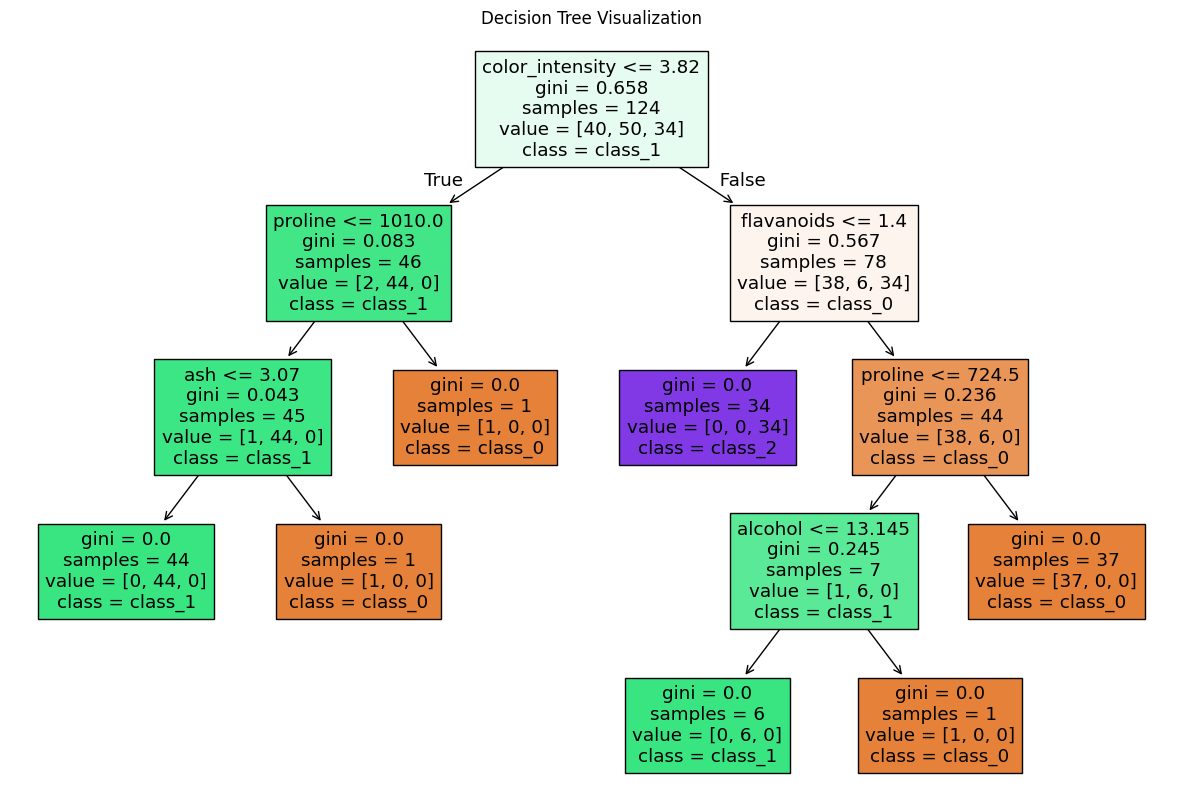
The model is making decisions by asking questions about the features. Each box shows the condition (for example, color intensity), the number of samples ( samples), number of samples per class (value) and the predicted class by majority (class). The gini value measures how mixed the classes are in a node, if it is closer to 0 the data is mostly one class. A high gini the data is more mixed.

Try different values of max_depth, min_samples_split. You can use GridSearchCV (remember to import the library)

# plot the tree

4. Random Forest

A Random Forest is an ensemble learning method that builds many decision trees and combines their predictions. Instead of relying on a single tree, trains multiple trees on different subsets of the data.

• n_estimators: Number of trees in the forest. More trees usually brings better performance.

• random_state: Controls randomness.

• max_depth: Maximum depth of each tree.

• min_samples_split: Minimum number of samples required to split a node.

• max_features: Number of features considered at each split. There are different options: sqrt(compute the square root), log2(compute the logarithm of the features \(log_2\)(features)), fixed number or a percentage

rf = RandomForestClassifier(n_estimators=100, random_state=42)

Let’s train the random forest:

rf.fit(X_train, y_train)

RandomForestClassifier(random_state=42)

In a Jupyter environment, please rerun this cell to show the HTML representation or trust the notebook.
On GitHub, the HTML representation is unable to render, please try loading this page with nbviewer.org.

Perform predictions:

y_pred_rf = rf.predict(X_test)

Evaluate the model:

print("Random Forest Accuracy:", accuracy_score(y_test, y_pred_rf))
print(classification_report(y_test, y_pred_rf))

Random Forest Accuracy: 1.0
              precision    recall  f1-score   support

           0       1.00      1.00      1.00        19
           1       1.00      1.00      1.00        21
           2       1.00      1.00      1.00        14

    accuracy                           1.00        54
   macro avg       1.00      1.00      1.00        54
weighted avg       1.00      1.00      1.00        54

Try different values of n_estimators,max_features, max_depth, min_samples_split. You can use GridSearchCV

4. XGBoost

XGBoost (Extreme Gradient Boosting) is an advanced ensemble learning algorithm based on boosting.

What is boosting?

Boosting is a machine learning technique that combines multiple weak models (usually small decision trees) to create a strong, accurate model. It trains a simple model, checks where it makes mistakes, gives more importance to those mistakes and trains a new model focusing on those errors. It repeats this process multiple times. Then, combines all the models into one final prediction.

The parameters used are:

• n_estimators: Number of trees or boosting rounds. The more trees, better learning but we risk to overfitting.

• max_depth: Maximum depth of each tree.

• learning_rate: Step size for updating predictions. Giving a small value (0.01), learns slowly but can obtain better accuracy. Using a large value, learns faster but can miss an optimal solution.

• eval_metric: Evaluation metric used during training. We have auc for binary classification, mlogloss is multiclass log loss and measures how well predicted the probabilities match the ture labels.

• random_state: Controls randomness.

• subsample: fraction of samples used per tree.

• colsample_bytree: Fraction of features (columns) used for each tree

• gamma: Minimum loss reduction required to make a split. Controls how strict the model is when creating splits. If we put a 0, the model splits more easily.

There are much more parameters available: Link to documentation

xgb = XGBClassifier(
    n_estimators=100,
    max_depth=3,
    learning_rate=0.1,
    eval_metric='auc',
    random_state=42
)

xgb.fit(X_train, y_train)

XGBClassifier(base_score=None, booster=None, callbacks=None,
              colsample_bylevel=None, colsample_bynode=None,
              colsample_bytree=None, device=None, early_stopping_rounds=None,
              enable_categorical=False, eval_metric='auc', feature_types=None,
              gamma=None, grow_policy=None, importance_type=None,
              interaction_constraints=None, learning_rate=0.1, max_bin=None,
              max_cat_threshold=None, max_cat_to_onehot=None,
              max_delta_step=None, max_depth=3, max_leaves=None,
              min_child_weight=None, missing=nan, monotone_constraints=None,
              multi_strategy=None, n_estimators=100, n_jobs=None,
              num_parallel_tree=None, objective='multi:softprob', ...)

In a Jupyter environment, please rerun this cell to show the HTML representation or trust the notebook.
On GitHub, the HTML representation is unable to render, please try loading this page with nbviewer.org.

y_pred_xgb = xgb.predict(X_test)

print("XGBoost Accuracy:", accuracy_score(y_test, y_pred_xgb))
print(classification_report(y_test, y_pred_xgb))

XGBoost Accuracy: 0.9814814814814815
              precision    recall  f1-score   support

           0       1.00      1.00      1.00        19
           1       0.95      1.00      0.98        21
           2       1.00      0.93      0.96        14

    accuracy                           0.98        54
   macro avg       0.98      0.98      0.98        54
weighted avg       0.98      0.98      0.98        54