LSTM and GRU

LSTM (Long Short-Term Memory)

LSTM was proposed by Hochreiter and Schmidhuber in 1997 as a solution to the vanishing gradient problem of simple RNNs. The key idea is to introduce a cell state \(c_t\): a long-term memory vector that flows along the sequence and that the network can learn to read, write, and erase selectively through three gates:

Forget gate \(f_t\): decides what information from the previous cell state is forgotten.
Input gate \(i_t\): decides what new information is written to the cell state.
Output gate \(o_t\): decides which part of the cell state is used to generate the hidden state \(h_t\).

\[f_t = \sigma(W_f \cdot [h_{t-1}, x_t] + b_f),\]

\[i_t = \sigma(W_i \cdot [h_{t-1}, x_t] + b_i),\]

\[\tilde{c}_t = \tanh(W_c \cdot [h_{t-1}, x_t] + b_c),\]

\[c_t = f_t \odot c_{t-1} + i_t \odot \tilde{c}_t,\]

\[o_t = \sigma(W_o \cdot [h_{t-1}, x_t] + b_o),\]

\[h_t = o_t \odot \tanh(c_t).\]

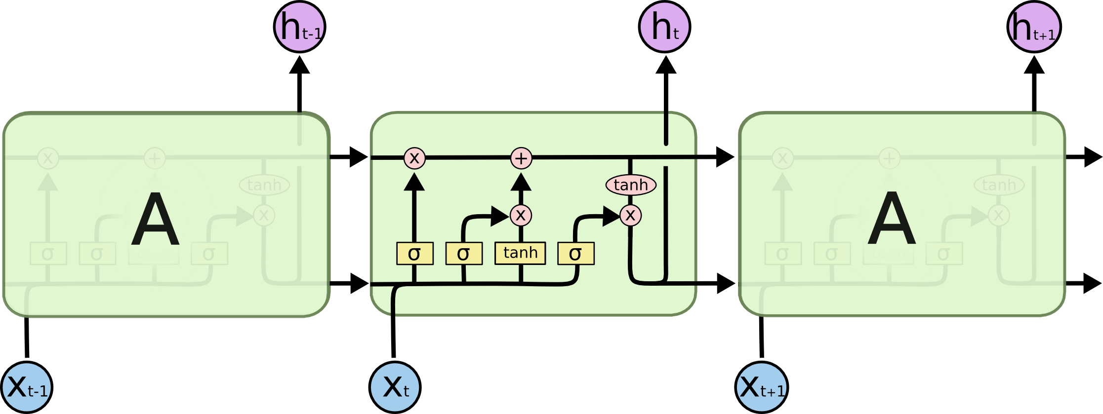
where \(\sigma\) is the sigmoid function and \(\odot\) is the element-wise product.

Parameters of `nn.LSTM`

nn.LSTM shares the same parameters as nn.RNN with one addition:

input_size: number of input variables at each time step.
hidden_size: dimension of the hidden state vector \(h_t\) and the cell state \(c_t\).
num_layers: number of stacked LSTM layers.
batch_first: if True, the input tensor is expected with shape [batch, seq_len, features].
dropout: applies dropout between layers when num_layers > 1.
bidirectional: if True, creates a bidirectional LSTM that processes the sequence in both directions.

Unlike nn.RNN, the forward method of nn.LSTM returns (out, (h_n, c_n)), i.e., both the hidden state and the cell state. This must be taken into account when defining the model’s forward method.

LSTM Model

import torch.nn as nn

class LSTMModel(nn.Module):
    def __init__(self, input_size=1, hidden_size=32, num_layers=1):
        super(LSTMModel, self).__init__()
        self.lstm = nn.LSTM(
            input_size=input_size,
            hidden_size=hidden_size,
            num_layers=num_layers,
            batch_first=True
        )
        self.fc = nn.Linear(hidden_size, 1)

    def forward(self, x):
        out, (h_n, c_n) = self.lstm(x) # difference with RNN
        out = self.fc(out[:, -1, :])  # take the last time step
        return out.squeeze()

GRU (Gated Recurrent Unit)

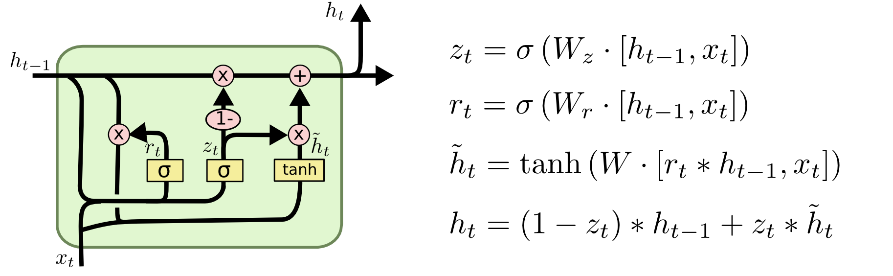
The GRU was proposed by Cho et al. in 2014 as a simplification of the LSTM. It eliminates the cell state and reduces the three gates to two:

Reset gate \(r_t\): controls how much information from the previous hidden state is discarded.
Update gate \(z_t\): controls how much of the previous hidden state is preserved and how much is replaced by new information.

\[r_t = \sigma(W_r \cdot [h_{t-1}, x_t] + b_r)\]

\[z_t = \sigma(W_z \cdot [h_{t-1}, x_t] + b_z)\]

\[\tilde{h}_t = \tanh(W_h \cdot [r_t \odot h_{t-1}, x_t] + b_h)\]

\[h_t = (1 - z_t) \odot h_{t-1} + z_t \odot \tilde{h}_t\]

Parameters of `nn.GRU`

nn.GRU has exactly the same parameters as nn.RNN:

input_size: number of input variables at each time step
hidden_size: dimension of the hidden state vector \(h_t\)
num_layers: number of stacked GRU layers
batch_first: if True, the input tensor is expected with shape [batch, seq_len, features]
dropout: applies dropout between layers when num_layers > 1
bidirectional: if True, creates a bidirectional GRU

Note: unlike LSTM, nn.GRU returns (out, h_n), without a cell state, just like nn.RNN.

GRU Model

class GRUModel(nn.Module):
    def __init__(self, input_size=1, hidden_size=32, num_layers=1):
        super(GRUModel, self).__init__()
        self.gru = nn.GRU(
            input_size=input_size,
            hidden_size=hidden_size,
            num_layers=num_layers,
            batch_first=True
        )
        self.fc = nn.Linear(hidden_size, 1)

    def forward(self, x):
        out, h_n = self.gru(x)
        out = self.fc(out[:, -1, :])  # take the last time step
        return out.squeeze()

Differences Between RNN, LSTM, and GRU

Let’s see the differences of these three types of recurrent modules:

	RNN	LSTM	GRU
Long-term memory	No	Yes (cell state)	Yes (update gate)
Number of gates	0	3	2
Parameters	Few	Many	Intermediate
Training speed	Fast	Slow	Intermediate
Vanishing gradient	Yes	No	No

When to Use Each One

RNN: short sequences where long-term memory is not needed. In practice, it is rarely the best option.

LSTM: when long-term dependencies are important and sufficient data and computational capacity are available. It is the default option for most time series problems.

GRU: when a good balance between performance and computational efficiency is desired. With small datasets or limited resources, it often gives results similar to LSTM with less training time.

Exercise: Comparison of RNN, LSTM, and GRU

Using the surface temperature (SST) time series dataset and the same data preparation as in the previous section, train an LSTM and GRU with the same architecture and experimental configuration and fill in the results table:

Model	MAE	RMSE	MAPE (%)
RNN
LSTM
GRU

Visualise the predictions of the three models in the same plot to facilitate comparison.